Probability Density Function Library In Solidity 

Paradigm recently put out a paper outlining the basics of what a ‘distribution market’ could look like. The difference between a distribution market and a normal prediction market is that instead of buying outcome tokens from a fixed set, you can bet over continuous outcomes. 

That means for a market like ‘How many people will attend the event?’, instead of being forced into options like A: <10,000 B: 10,000 - 20,000 etc, you can say I think 12,345 +/-2,000 people will attend.

To do this we needed to translate the traders bet and confidence into an equation that could generate a distribution of points over some interval - ie we needed a probability density function. 

When I looked to see if any probability density function (PDF) libraries existed, there were 3 main stand alone repos in solidity.

1. Solstat: Primitive Finance

2. Statistics Solidity: DeltaDex Protocol

3. Solgauss: Cairo.eth

All the libraries are useful and work under certain conditions, but they lacked some features that we needed.

Our ideal library needed:

• To generate PDFs for a range of $$\mu$$ and $$\sigma$$ . The constraint of $$\mu=0$$,

  $$\sigma=1$$ was too restrictive.

• To be able to operate on different scales. So people can predict values on the order of $$10$$ or $$10\space eth$$

• Utilities to relate multiple PDFs (like finding the point of maximum difference between 2 PDFs)

• A test framework that could link to our other code related to the distribution market.

Solidity does not have built in support for floating point math, so any values that have decimals would get cut off. The worst form of this is when a number is a decimal less than 1, which just gets rounded to 0, something that is obviously bad for a PDF which has terms like $$\frac{1}{\sigma\sqrt2\pi}$$.

To get around this we scale all our numbers up and work in ‘fixed point math’ where we assume a huge number like $$1e^{18}$$ actually equals 1. That’s great because now instead of rounding numbers like $$\pi\approx3$$ we can do

$$\pi=3.141592653589793238 * 1e^{18} = 3141592653589793238$$

So any time we see a number like that, we need to remember the amount we scaled it by, and be careful to either operate on that scale, or convert it back down offchain. Scaling numbers like this is straightforward when we just want to do simple operations like adding or dividing numbers. But the PDF is not so simple, and if we are to work with scaled numbers, we need to see how it behaves for different inputs. 

$$ p(x) = \frac{1}{\sigma\sqrt{2\pi}} e^{-\frac{1}{2}\left(\frac{x-\mu}{\sigma}\right)^2} $$

Looking at the above equation and thinking back to our original example of predicting attendees at an event, we can gain some understanding of how the PDF should scale. If we consider a normal event to have 100 attendees $$\pm20$$, then we can work out the probability that x people will show up. One thing to notice is that since all those parameters are measured in attendees, if we scale things, then scaling all of the parameters by the same amount makes sense.

Since the exponent $${-\frac{1}{2}\left(\frac{x-\mu}{\sigma}\right)^2}$$ has equal orders of scaling in the numerator and denominator, any scaling cancels out. The coefficient has a sigma in the denominator, meaning that scaling the inputs will produce a much smaller peak. This aligns with the normalisation constraint on PDFs, $$\int_{-\infty}^{\infty}{p(x)}dx=1$$, since when we stretch the range with our scaling, the height must get smaller to keep the area the same.

But in Solidity we are actually going to be working in fixed point math where $$1e^{18}=1$$, so we need to scale our inputs to convert them to this number system, and also need to consider the other constants like $$2$$ and $$\pi$$ in the same way. This is why we use a library like Prb-Math.

Since we want to be able to work with negative numbers, we choose the (signed decimal) SD59x18 number type from PRB-Math. This lets us operate with 59 integer numbers and 18 decimals by representing those numbers in the range of an int256.

/// User defined type to ensure we know we are operating with a custom number type, not int256
type SD59x18 is int256;
// Upper bound is type(int256).max
int256 constant uMAX_SD59x18 = 57896044618658097711785492504343953926634992332820282019728_792003956564819967;
// Lower bound is type(int256).min
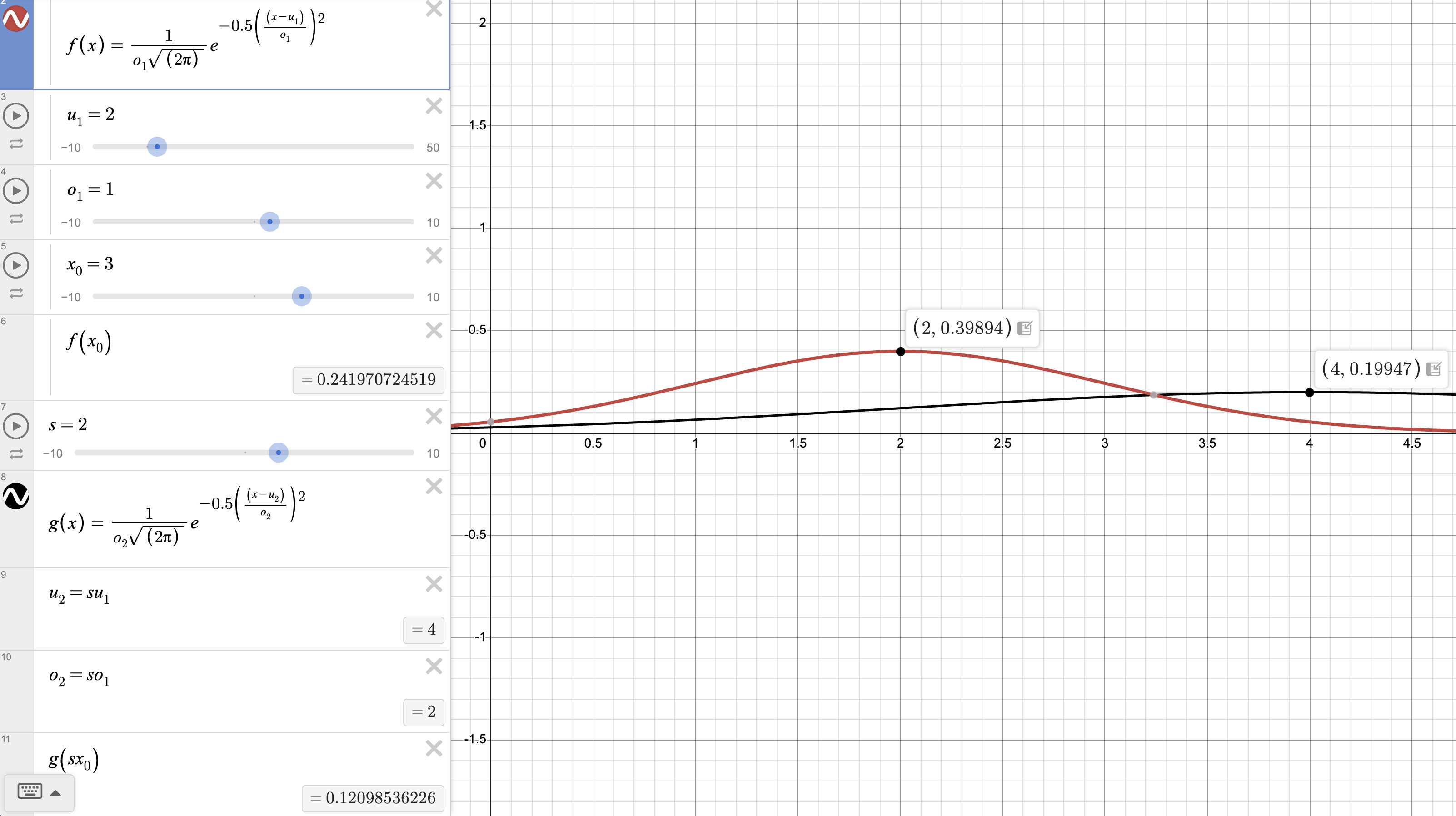
int256 constant uMIN_SD59x18 = -57896044618658097711785492504343953926634992332820282019728_792003956564819968;

Using this number type allows us allows us to calculate the PDF from the $$f(x)$$ curve in the Desmos graph above for inputs: $$x=3, \mu=2, \sigma=1$$

function pdf(SD59x18 x, SD59x18 mean, SD59x18 sigma) returns (SD59x18 p) {
/// x - µ = 1e^18
SD59x18 xMinusMean = x - mean;
/// -(x - µ)^2 = -1e^18
SD59x18 exponentNumerator = -xMinusMean.pow(TWO);
/// 2σ^2 = 2e^18
SD59x18 exponentDenominator = TWO.mul(sigma.pow(TWO));
/// full exponent = -5e^17
SD59x18 exponentFull = exponentNumerator.div(exponentDenominator);
/// e^((-(x - µ)^2) / 2σ^2) = 6.07e17
SD59x18 exponentResult = exp(exponentFull);
/// σ√2π = 2.51e18
SD59x18 denominator = sigma.mul(SQRT_2PI);
/// 1 / σ√2π = 3.99e^17
SD59x18 coefficient = inv(denominator);
/// p = (1 / σ√2π)e^((-(x - µ)^2) / 2σ^2) = 2.42e^17
p = mul(coefficient, exponentResult)
}

As you can see the result is $$2.42e^{17}$$ , which if you consider $$1e^{18}=1$$, is the same as saying $$0.242$$. This agrees with Desmos and shows that we don't have to lose precision when working with decimals in Solidity.

The library includes the following functions:

• pdf: The probability density function

• pdfDifference: The difference between two pdfs

• isMinimumPoint: Checks if a point is the minimum point of a curve given by pdf2 - pdf1

• isMaximumPoint: Checks if a point is the maximum point of a curve given by pdf2 - pdf1

• pdfDerivativeAtX: The first derivative of a pdf at a given x

• pdfSecondDerivativeAtX: The second derivative of a pdf at a given x

  These functions have wrappers like the below to receive values in int256, so you don't need to import any Prb-Math types into your code to get values back.

    function pdf(int256 x, int256 mean, int256 sigma) internal pure returns (int256) {
        return pdf(convert(x), convert(mean), convert(sigma)).unwrap();
    }

All tests are run against reference PDF values calculated in typescript like the below.

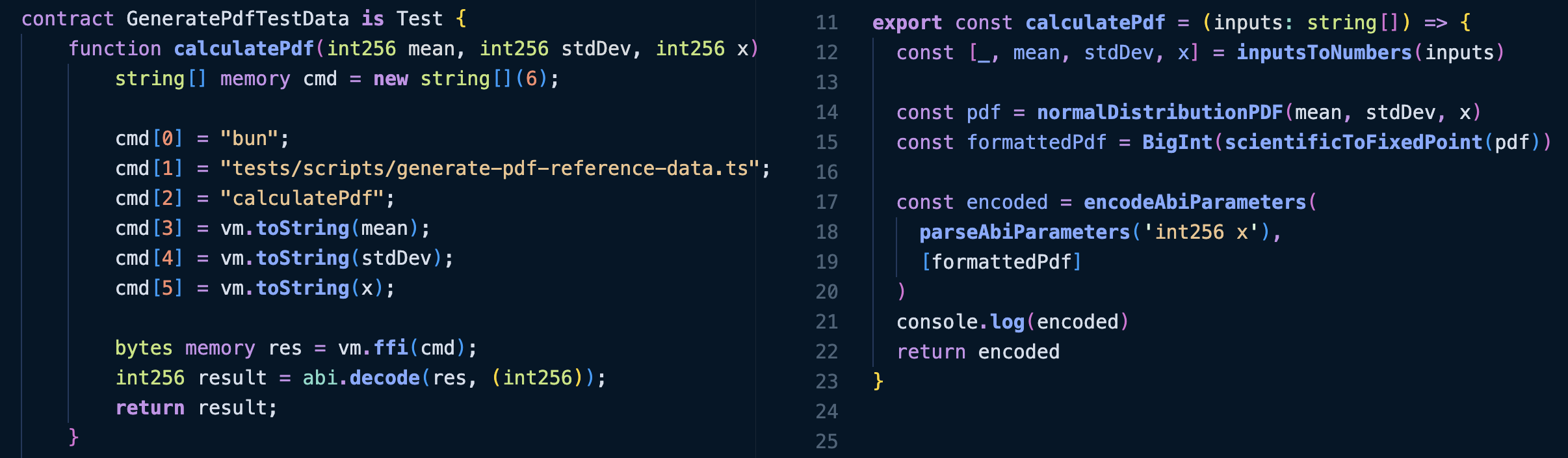
You can find the code here and if you have any questions drop me a message on farcaster